You can connect with me on LinkedIn to discuss collaborations and work opportunities.
pandas 3.0 has just been released. This article uses a real‑world example to explain the most important differences between pandas 2 and the new pandas 3 release, focusing on performance, syntax, and user experience.
A note on pandas versioning
Before diving into the technical details of pandas 3, it is worth providing some context on how pandas is developed and what to expect from its release cycle.
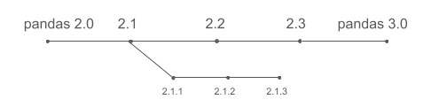
Many software projects develop new features in parallel between major releases. If pandas followed this model, development might look like this:
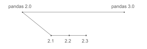
This is often what users expect. In reality, pandas development follows a different approach:
pandas does not develop features in parallel across major versions. Instead, new features land continuously on the main development line and are included in the next release once they are ready (for example 2.1). As a result, pandas 3.0 does not include everything developed since pandas 2.0 (released almost three years ago), but primarily what has been added since pandas 2.3, which was released roughly six months ago.
Most importantly, the pandas developers consistently prioritize backward compatibility. Instead of continuously breaking APIs to improve everything that can be improved, we aim to fix what can reasonably be fixed without forcing users to rewrite their codebases. Users maintaining large pandas projects, or those who simply do not want to relearn pandas syntax every year, will likely appreciate this philosophy.
The downside of this conservative approach is that pandas cannot always offer state‑of‑the‑art performance or a clean and consistent API, and instead will suffer from some design decisions that made sense a couple of decades ago, but that we would implement differently if we started pandas today. For users starting fresh with dataframe‑based projects, it is worth considering Polars, which could learn from pandas experience to deliver a dataframe library with impressive performance, full Arrow support, and a cleaner and more consistent API.

That said, pandas 3 still introduces several significant changes that improve performance, syntax, and the overall user experience. Let’s take a closer look.
The pandas warning from hell
The examples in this article use a dataset containing 2,231,577 hotel room records, with the following structure:
| name | country | property_type | room_size | max_people | max_children | is_smoking |
|---|---|---|---|---|---|---|
| Single Room | it | guest_house | 15.0503 | 1 | 0 | False |
| Single Room Sea View | gr | hotel | 19.9742 | 1 | 0 | False |
| Double Room with Two Double Beds – Smoking | us | lodge | 32.5161 | 4 | 3 | True |
| Superior Double Room | de | hotel | 19.9742 | 2 | 1 | False |
| Single Bed in Female Dormitory Room | br | hostel | 6.0387 | 1 | 0 | False |
We will start with pandas 2. Our first operation is to add the maximum number of children a room can accommodate to the maximum number of people (adults), but only for U.S. hotels.
>>> all_rooms = pandas.read_parquet("rooms.parquet")
>>> us_hotel_rooms = all_rooms[(all_rooms.property_type == "hotel") & (all_rooms.country == "us")]
>>> us_hotel_rooms["max_people"] += us_hotel_rooms.max_children
This produces the infamous warning:
SettingWithCopyWarning:
A value is trying to be set on a copy of a slice from a DataFrame.
Try using .loc[row_indexer,col_indexer] = value instead

See the caveats in the documentation: https://pandas.pydata.org/pandas-docs/stable/user_guide/indexing.html#returning-a-view-versus-a-copy
  us_hotel_rooms["max_people"] += us_hotel_rooms.max_children
If you have used pandas for any length of time, you have almost certainly seen this before. What is happening can be summarized as follows:
us_hotel_roomscould be very large, imagine 10 GB in memory.- Copying those 10 GB would be slow and require another 10 GB of RAM.
- Ideally, pandas would like to avoid the copy and instead keep a
reference to the relevant rows of
all_rooms. - This becomes problematic when the user mutates
us_hotel_rooms, since that mutation could unexpectedly affectall_rooms. - pandas 2 uses complex heuristics to decide whether a copy is created, and the warning exists to signal that unexpected side effects may occur.
In practice, most users do not fully understand the underlying issue and handle the warning in one of two ways (often based on advice from StackOverflow or a chatbot):
- Suppress the warning globally with
warnings.filterwarnings("ignore"). - Consistently copy after every operation using
df = df.copy().
The standard solution to this class of problems is copy‑on‑write:
- Never copy data eagerly after filtering.
- Automatically create a copy only when a dataframe that references another dataframe is mutated.
After countless hours of work that began well before pandas 3, copy‑on‑write is
now fully implemented. The warning is gone, and all the .copy() calls in pandas
code can be safely avoided after moving to pandas 3.
Improved pandas syntax
Let's revisit the same example, this time focusing on syntax rather than memory behavior. For users who write pandas pipelines rather than interactively exploring data in a notebook, the previous example can be rewritten using method chaining:
(
    pandas.read_parquet("rooms.parquet")
          [lambda df: (df.property_type == "hotel") & (df.country == "us")]
          .assign(max_people=lambda df: df.max_people + df.max_children)
)
This style avoids repeated assignments and makes the sequence of operations explicit.
However, while method chaining itself makes the code more readable, many users will find
this version harder to read, largely because of the required use of lambda,
which is a non‑trivial pandas concept.
In pandas, column access typically uses either df.column or df["column"].
With method chaining, however, the intermediate DataFrame object does not exist as a
named variable at each step. Even if we create df, the df in the assign operation
is not the DataFrame object at the time of assigning (with only U.S. hotel data), but
the original DataFrame with all rows:
df = pandas.read_parquet("rooms.parquet")

df = (
    df[(df.property_type == "hotel") & (df.country == "us")]
      .assign(max_people=df.max_people + df.max_children)
)
The use of lambda delays evaluation so that column expressions are resolved
against the correct intermediate DataFrame. While effective, this approach using
lambda makes reading pandas code significantly harder. Other libraries such as
Polars and PySpark address this more cleanly using a col() expression API.
pandas 3 introduces the same mechanism:
(
    pandas.read_parquet("rooms.parquet")
          [(pandas.col("property_type") == "hotel") & (pandas.col("country") == "us")]
          .assign(max_people=pandas.col("max_people") + pandas.col("max_children"))
)
This is a significant step forward, making pandas code much more readable, in particular when using method chaining. But there is still room for improvement. For comparison, the equivalent filter in Polars looks like this:
.filter(polars.col("property_type") == "hotel", polars.col("country") == "us")
Using an explicit .filter() method makes the operation being performed clearer.
Experienced Python developers will be familiar with Tim Peter's brilliant
Zen of Python which states that
"explicit is better than implicit". Using df[...] for both filtering and selection is
surely convenient, more in interactive use, but it can become confusing in chained pipelines.
More importantly, pandas still relies on the bitwise & operator for combining conditions.
Ideally, users would write condition1 and condition2, but Python reserves and for
boolean evaluation and does not allow libraries to override it.
Using & leads to this surprising behavior:
>>> 1 == 1 & 2 == 2
False
The expression is evaluated as 1 == (1 & 2) == 2, not (1 == 1) and (2 == 2).
The same happens when each side of the & is a pandas expression. This is why in the previous
example [(pandas.col("property_type") == "hotel") & (pandas.col("country") == "us")]
conditions must be carefully parenthesized.
Since overriding and, or, and not is not possible in Python, and not likely to be allowed
anytime soon, the Polars approach is probably the best it can be done. Implementing .filter() and
allowing passing multiple conditions as different arguments is something that could be
implemented in pandas, and will hopefully be available to users in a future version.
Accelerated pandas functions
Another important improvement in pandas 3 is better support for user‑defined functions (UDFs).
In pandas, UDFs are regular Python functions passed to methods such as .apply() or .map().
If you have used pandas for a while, you have probably heard that .apply() is considered bad practice:

This reputation is often deserved. For example, adding max_people and max_children row‑by‑row:
def add_people(row):
    return row["max_people"] + row["max_children"]

rooms.apply(add_people, axis=1)
produces the same result as the vectorized version, but increases execution time from roughly 3 ms to 11 seconds (around 4,000x slower).
However, not all problems vectorize cleanly. Consider transforming a room name such as "Superior Double Room with Patio View" into a structured string like:
property_type=hotel, room_type=superior double, view=patio
A fully vectorized solution quickly becomes complex and hard to maintain. This implementation takes around 14 seconds with the example dataset:
name_lower = df["name"].str.lower()
before_with = name_lower.str.split(" with ").str[0]
after_with = name_lower.str.split(" with ").str[1]

view = (("view=" + after_with.str
                             .removesuffix(" view"))
                             .where(after_with.str.endswith(" view"),
                                    ""))
bathroom = (("bathroom=" + after_with.str
                                     .removesuffix(" bathroom"))
                                     .where(after_with.str.endswith(" bathroom"),
                                            ""))
result = (
    "property_type="
    + df["property_type"]
    + ", room_type="
    + before_with.str.removesuffix(" room")
    + pandas.Series(", ", index=before_with.index).where(view != "", "")
    + view
    + pandas.Series(", ", index=before_with.index).where(bathroom != "", "")
    + bathroom
)
The equivalent UDF is (at least in my opinion) far clearer:
def format_room_info(row):
    result = "property_type=" + row["property_type"]

    desc = row["name"].lower()
    if " with " not in desc:
        return result + ", room_type=" + desc.removesuffix(" room")

    before, after = desc.split(" with ", 1)
    result += ", room_type=" + before.removesuffix(" room")

    if after.endswith(" view"):
        result += ", view=" + after.removesuffix(" view")
    elif after.endswith(" bathroom"):
        result += ", bathroom=" + after.removesuffix(" bathroom")

    return result


df.apply(format_room_info, axis=1)
This version runs in about 22 seconds, roughly 70% slower than the vectorized approach, but is far easier to read and maintain.
pandas 3 introduces a new execution interface that allows third‑party engines to accelerate UDFs. One example is bodo.ai, which can JIT‑compile both pure Python and pandas code:
import bodo

df.apply(format_room_info, axis=1, engine=bodo.jit())
With bodo.ai, the same code runs in around 9 seconds, less than half of the time needed with the standard UDF version, and also 35% faster than the vectorized version. And this speed-up is gained while retaining the clarity of the UDF implementation.
Although a 35% speed‑up may not sound dramatic, JIT compilation has a fixed startup cost, the time to compile the code, which does not depend on the amount of data processed later. As datasets grow larger, the relative gains increase substantially. For very large datasets, the difference can be dramatic. So, in this example, if we had 100 million rows instead of 2, using bodo.ai would improve performance massively.
Crucially, execution now happens outside pandas itself. This opens the door
to an ecosystem of specialized execution engines. For example,
Blosc can accelerate NumPy‑style
workloads using compressed memory execution, and works with pandas 3 as
simply as bodo, just by using engine=blosc2.jit(). Enabling this ecosystem
adds endless possibilities. For example, bodo.ai also supports distributed
execution on HPC clusters, and other engines may emerge for different use-cases
and different strategies.
What happened to the Apache Arrow revolution?
If you read my earlier article pandas 2.0 and the Arrow revolution, you may be wondering what became of that effort.
At the time pandas 2 was being released, the core team was committed to implement a more aggressive transition to Apache Arrow. Primarily, to make sure users could always benefit from the performance and compatibility enhancements Arrow provides. This would be particularly relevant for strings, where the legacy implementation is really suboptimal compared to the Arrow one. Ultimately, this plan was scaled back. This is in short what happened:
- PyArrow was initially planned as a required dependency. Without this point, legacy strings can't be fully replaced.
- Users were shown a warning about the upcoming requirement during a short period of time.
- Feedback raised concerns, mostly about disk usage, and platform support.
- A hybrid approach was proposed, where users with PyArrow installed would have
strings backend by Arrow by default. And users without PyArrow would continue
to use the legacy strings. But this change would be implemented in a mostly
transparent way for users. In both cases, strings would use a new
strdata type, and missing values would behave like in the legacyNaNrepresentation. - This proposal was approved, and even after PyArrow addressed most of the initial concerns, making it mandatory was abandoned, and the hybrid approach was implemented
With an example, the new strings look like this:
>>> pandas.Series([None, "a", "b"])
0    NaN
1      a
2      b
dtype: str

>>> pandas.Series([None, "a", "b"]) == "a"
0    False
1     True
2    False
dtype: bool
In the example, the data type is the new str type, and the missing value is
represented by NaN, and when comparing NaN == "a" the return is False.
You can't know whether the code above uses NumPy's objects internally, or
Arrow strings, since that depends on the environment and not the code itself.
By contrast, the pure Arrow approach looks like this:
>>> pandas.Series([None, "a", "b"], dtype="string[pyarrow]")
0    <NA>
1       a
2       b
dtype: string

>>> pandas.Series([None, "a", "b"], dtype="string[pyarrow]") == "a"
0     <NA>
1     True
2    False
dtype: bool[pyarrow]
Missing values are not the float NaN anymore but pandas <NA> which is not
exactly a value itself, but a reference to whether the value is missing or not.
In Arrow, a separate array is used to establish which values are missing.
The main difference in the example is that <NA> == "a" in this case returns
<NA> and not False as the default pandas 3 implementation.
I'm not personally aware of any current plan or effort to change the pandas 3
status quo significantly. While the new approach is a good trade-off between
backward compatibility and allowing users to benefit from Arrow by default, it
comes with its drawbacks. Now there are 3 different ways to represent strings,
since the PyArrow example above is still valid in pandas 3, as it would be
setting dtype="object" and using the original implementation. It may also not
be ideal for some users to have the same code running with different implementation
depending on whether PyArrow is installed or not. This can be tricky for example
for developers of other libraries, who can't make assumptions on what a pandas
string is internally.
Clearly, the users that will benefit more from the new pandas 3 strings are users with existing codebases concerned about backward compatibility. While the new changes are not fully backward compatible, migrating to pandas 3 should be really straightforward.
Users who need a simpler and modern dataframe experience based on Arrow, and are less concerned about pandas legacy, Polars is a great alternative.